Finding the perfect sock pattern with {ravelRy}

I am a knitter. Knitting is a calming, fulfilling practice that keep my hands busy and require just enough brain power to keep my mind from wandering too far. Over the past winter, I conquered my fear of making socks, and now I profess that I am a sock knitter. I made socks for Christmas gifts, and churned out four pairs during my evenings, bus commutes, long work meetings, lectures, coffee and tea shop visits (basically everywhere). I’m comfortable with the standard stockinette sock, and I even ventured out into other patterns from Ravelry (the social medium for yarn folks), like Hermione’s Everyday Socks and the Slip It Simple Socks.
But, even as the weather is warming here in Minnesota, working from home means that I don’t have a commute and COVID-19 means that I have plenty of spare angst, so I’ve decided to make a new pair of socks, and work with a new pattern.
And, just when I was starting to glaze over scrolling through endless Ravelry pages and reviews, I found ravelRy, an R package that interfaces seamlessly with Ravelry’s API. And its even on CRAN!
Lets install, and get going!
install.packages("ravelRy")
library(ravelRy)
library(tidyverse)
Authentication
As with most APIs, you need to authenticate somehow. I’ll use my Ravelry account credentials (you’ll need a free, pro account to access the API).
ravelRy::ravelry_auth(key = "username")
ravelRy::ravelry_auth(key = "password")
Search for a sock pattern!
Lets start simple, and just look for the first 20 results for “sock” that are available as a Ravelry download.
search_result <- search_patterns(
  query = "sock",
  page_size = 20,
  craft = "knitting", # knitting or crochet
  fit = "adult", # adult, baby, etc.
  ravelry_download = TRUE
)

head(search_result)
#> # A tibble: 6 x 7
#>   free       id name         permalink designer.id designer.name pattern_sources
#>   <lgl>   <int> <chr>        <chr>           <int> <chr>         <list>
#> 1 FALSE 1222621 Engelkrista~ engelkri~       34635 Caia Gossens  <df [2 x 60]>
#> 2 TRUE  1250944 Vecna        vecna           97793 Dots Dabbles  <df [1 x 60]>
#> 3 FALSE 1229788 Plaid Pocke~ plaid-po~      111830 Shuyi Wu      <df [2 x 60]>
#> 4 TRUE  1235715 Cably Wably  cably-wa~       32564 Liz Sedmak    <df [2 x 60]>
#> 5 FALSE 1091238 DRK Everyda~ drk-ever~       78156 Andrea Mowry  <df [1 x 60]>
#> 6 TRUE  1244939 Sock Prince~ sock-pri~       92088 Annette Schl~ <df [1 x 60]>
The fourth result is even my old friend, “Hermione’s Everyday Socks!”
search_result[4, ] # get the fourth row in the table
#> # A tibble: 1 x 7
#>   free       id name        permalink  designer.id designer.name pattern_sources
#>   <lgl>   <int> <chr>       <chr>            <int> <chr>         <list>
#> 1 TRUE  1235715 Cably Wably cably-wab~       32564 Liz Sedmak    <df [2 x 60]>
Lets take a look at the actual pattern from the search results using get_patterns().
hermione <- get_patterns(ids = search_result[4, ]$id)
str(hermione, max.level = 2)
#> tibble [1 x 50] (S3: tbl_df/tbl/data.frame)
#>  $ comments_count         : int 4
#>  $ created_at             : chr "2022/04/19 09:02:36 -0400"
#>  $ currency               : chr "USD"
#>  $ difficulty_average     : num 6.36
#>  $ difficulty_count       : int 150
#>  $ downloadable           : logi FALSE
#>  $ favorites_count        : int 428
#>  $ free                   : logi TRUE
#>  $ gauge                  : num 8
#>  $ gauge_divisor          : int 1
#>  $ gauge_pattern          : chr "stockinette stitch"
#>  $ generally_available    : chr "2022/04/01 00:00:00 -0400"
#>  $ id                     : int 1235715
#>  $ name                   : chr "Cably Wably"
#>  $ pdf_url                : chr ""
#>  $ permalink              : chr "cably-wably"
#>  $ price                  : chr ""
#>  $ projects_count         : int 848
#>  $ published              : chr "2022/04/01"
#>  $ queued_projects_count  : int 55
#>  $ rating_average         : num 4.55
#>  $ rating_count           : int 152
#>  $ row_gauge              : num 11
#>  $ updated_at             : chr "2022/06/09 18:40:59 -0400"
#>  $ url                    : chr ""
#>  $ yardage                : int 350
#>  $ yardage_max            : int 500
#>  $ personal_attributes    : chr ""
#>  $ sizes_available        : chr "Small (8.5”, 21.5 cm) (Large (9.5”, 24 cm)) actual circumference"
#>  $ product_id             : chr ""
#>  $ currency_symbol        : chr "$"
#>  $ ravelry_download       : logi FALSE
#>  $ download_location      : chr ""
#>  $ pdf_in_library         : logi FALSE
#>  $ volumes_in_library     : chr ""
#>  $ gauge_description      : chr "8 stitches and 11 rows = 1 inch in stockinette stitch"
#>  $ yarn_weight_description: chr "Fingering (14 wpi)"
#>  $ yardage_description    : chr "350 - 500 yards"
#>  $ pattern_needle_sizes   :List of 1
#>  $ notes_html             : chr "\n<p>These socks were designed for Round 3 of the 2022 Sock Madness competition and will be exclusive to the pl"| __truncated__
#>  $ notes                  : chr "These socks were designed for Round 3 of the 2022 Sock Madness competition and will be exclusive to the players"| __truncated__
#>  $ packs                  :List of 1
#>  $ printings              :List of 1
#>  $ yarn_weight            :List of 1
#>  $ craft                  :List of 1
#>  $ pattern_categories     :List of 1
#>  $ pattern_attributes     :List of 1
#>  $ pattern_author         :List of 1
#>  $ photos                 :List of 1
#>  $ pattern_type           :List of 1
str(hermione$pattern_attributes)
#> List of 1
#>  $ : tibble [16 x 2] (S3: tbl_df/tbl/data.frame)
#>   ..$ id       : int [1:16] 3 10 12 18 22 25 56 64 204 207 ...
#>   ..$ permalink: chr [1:16] "unisex" "adult" "negative-ease" "fitted" ...
I thought the Hermione sock was fairly straightforward. What is the average difficulty, on a scale of 1 to 10?
hermione$difficulty_count # how many reviews rated a difficulty?
#> [1] 150
hermione$difficulty_average # what is the average difficulty?
#> [1] 6.36
Lets find my other sock pattern, Slip It Simple, and see what the difficulty rating is.
slip_it_search <- search_patterns(query = "slip it simple sock")
Next, take the id column and feed it into get_patterns().
slip_it <- get_patterns(ids = slip_it_search$id)
What is our difficulty?
slip_it$difficulty_count
#> [1]  67 102
slip_it$difficulty_average
#> [1] 2.447761 2.166667
There are fewer reviews, but the difficulty is super low.
Refining our search
We can use the pattern table for hermione and slip_it to narrow our search further.
head(search_patterns(
  query = "sock",
  page_size = 20,
  craft = "knitting", # knitting or crochet
  fit = "adult", # adult, baby, etc.
  ravelry_download = TRUE,
  pattern_needle_sizes = 1,
  weight = "fingering", # yarn weight
  type = "sock",
  colors = 1
))
...
#> # A tibble: 6 x 7
#>   free       id name         permalink designer.id designer.name pattern_sources
#>   <lgl>   <int> <chr>        <chr>           <int> <chr>         <list>
#> 1 TRUE  1235715 Cably Wably  cably-wa~       32564 Liz Sedmak    <df [2 x 60]>
#> 2 FALSE 1091238 DRK Everyda~ drk-ever~       78156 Andrea Mowry  <df [1 x 60]>
#> 3 FALSE 1121082 Senbonzakura senbonza~       31024 Natalia Vasi~ <df [2 x 60]>
#> 4 FALSE 1249732 Barleycorn   barleyco~      107022 Eva Romeijn   <df [1 x 60]>
#> 5 TRUE   891114 Rye Light    rye-light       45502 tincanknits   <df [3 x 60]>
...
Another trick is to go look at the URL when I am searching on Ravelry itself. This gives me an idea of what search terms I can add to search_patterns().
refined_search <- search_patterns(
  query = "socks",
  pc = "mid-calf",
  page_size = 100,
  craft = "knitting", # knitting or crochet
  # fit = "adult", # adult, baby, etc.
  ravelry_download = TRUE,
  pattern_needle_sizes = 1,
  weight = "fingering", # yarn weight
  type = "sock",
  colors = 1,
  diff = "3.5%7C8",
  language = "en",
  sort = "projects",
  photo = "yes"
)
Review refined search results
Now that I’ve picked out 100 patterns to consider/make fun plots with, lets review them in more detail.
refined_patterns <- get_patterns(ids = refined_search$id) # this might take a while
To start plotting, I will import my theme and {dutchmasters}.
source("my_sock_theme.R")
library(dutchmasters)
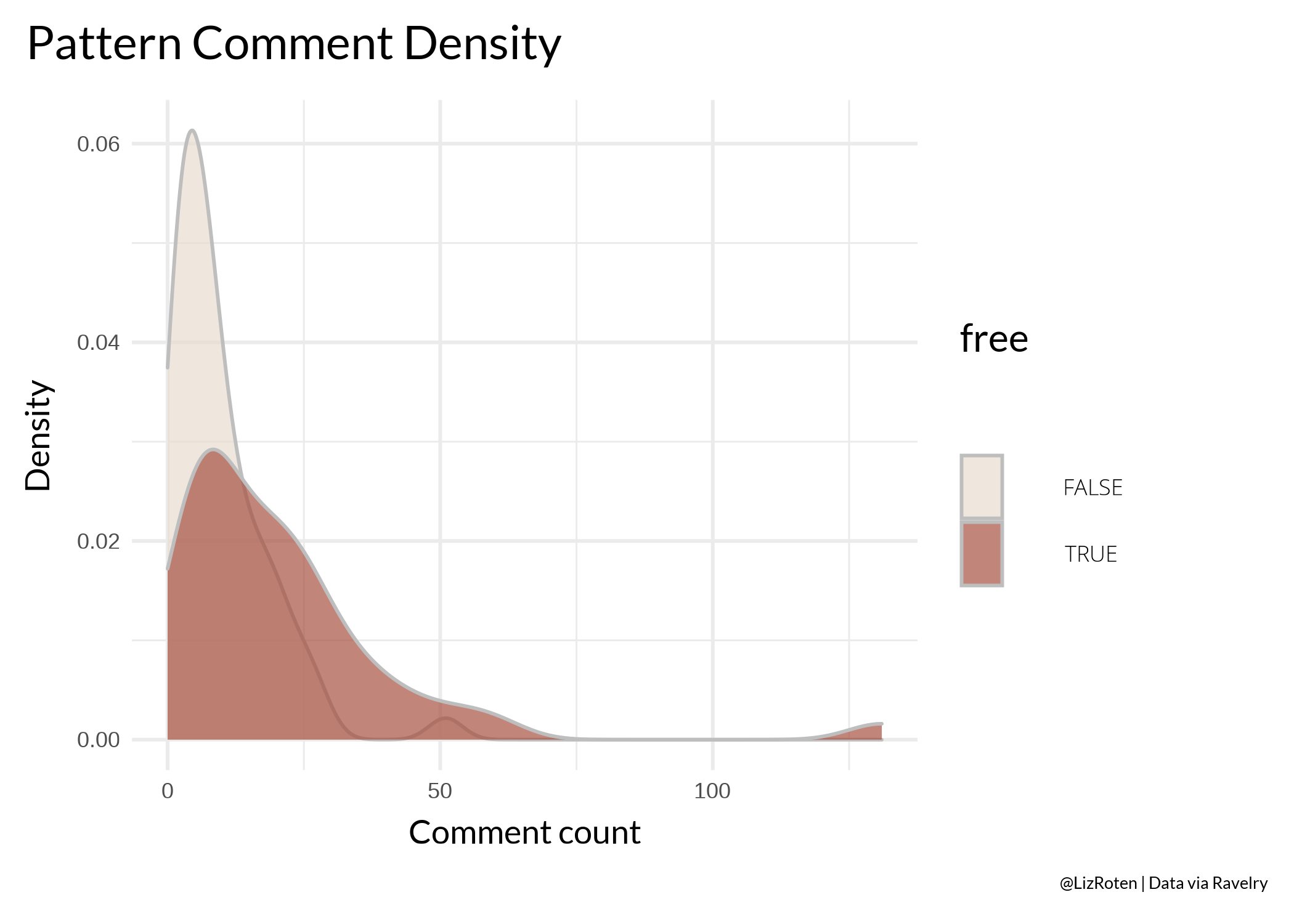
ggplot() +
  geom_density(refined_patterns,
    mapping = aes(
      x = comments_count,
      fill = free
    ),
    alpha = 0.7,
    color = "gray"
  ) +
  dutchmasters::scale_fill_dutchmasters(palette = "pearl_earring") +
  labs(
    title = "Pattern Comment Density",
    x = "Comment count",
    y = "Density",
    caption = my_caption
  ) +
  my_theme()
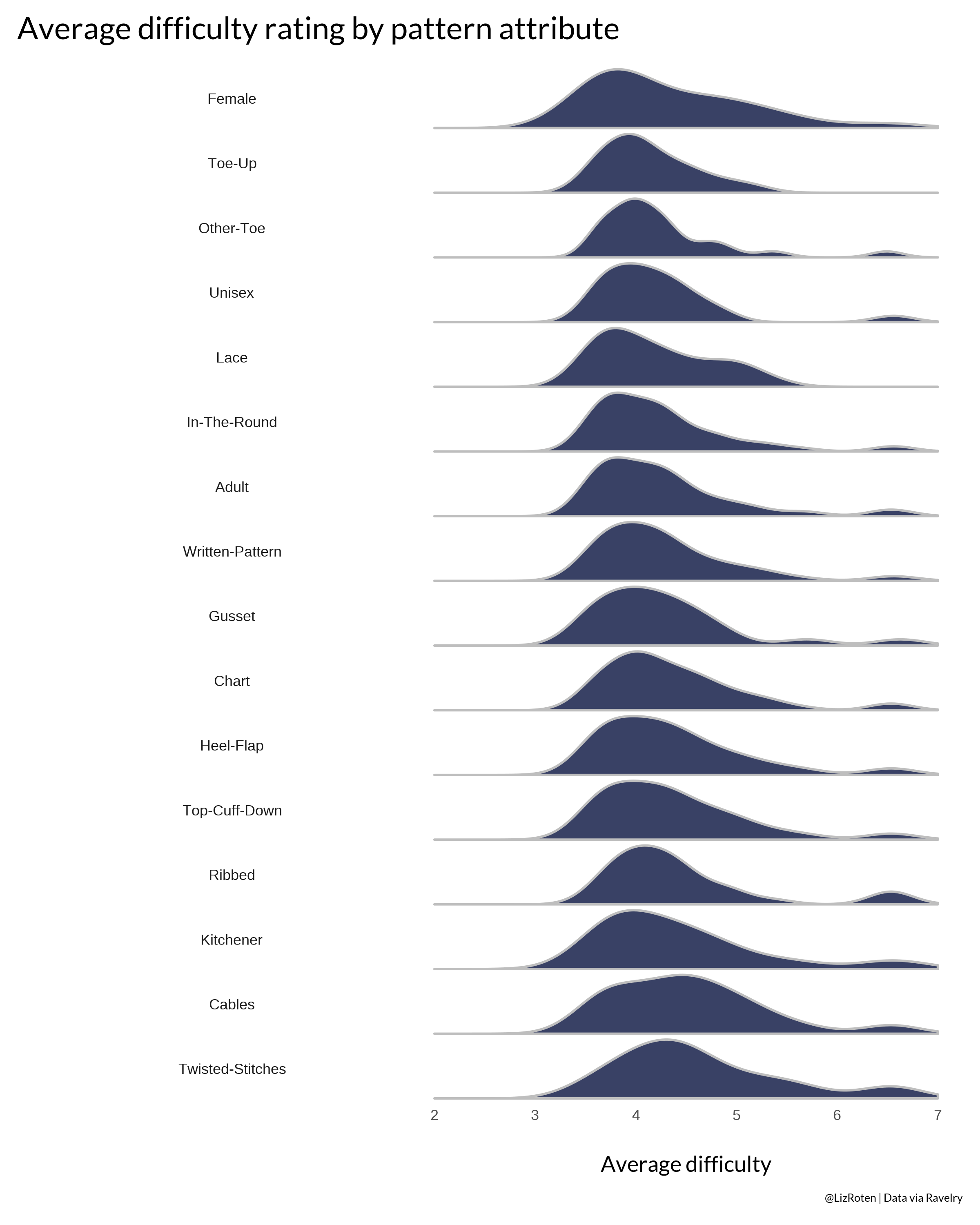
Next, we’ll make a density plot series comparing the average difficulty rating for each pattern attribute (check out this example for this plot’s inspiration).
pattern_details_attributes <- refined_patterns %>%
  unnest(cols = "pattern_attributes", names_sep = "_")


top_attributes <- pattern_details_attributes %>%
  filter(difficulty_count >= 20) %>%
  count(pattern_attributes_permalink) %>%
  filter(n >= 20)

attributes_long <- pattern_details_attributes %>%
  filter(pattern_attributes_permalink %in% top_attributes$pattern_attributes_permalink) %>%
  mutate(pattern_attributes_permalink = stringr::str_to_title(pattern_attributes_permalink)) %>%
  select(id, pattern_attributes_permalink, difficulty_average, rating_average)

plot_diff_by_att <- attributes_long %>%
  ggplot() +
  geom_density(aes(x = difficulty_average),
    fill = dutchmasters::dutchmasters$pearl_earring[4],
    color = "gray",
    outline.type = "full"
  ) +
  facet_grid(reorder(
    pattern_attributes_permalink,
    difficulty_average, median
  ) ~ .,
  switch = "y", scales = "free_y"
  ) +
  scale_x_continuous(limits = c(2, 7)) +
  labs(
    title = "Average difficulty rating by pattern attribute",
    # subtitle = "Sock knitting patterns",
    y = "", x = "Average difficulty",
        caption = my_caption

  ) +
  my_theme() +
  theme(
    panel.spacing.y = unit(0, "lines"),
    panel.grid = element_blank(),
    panel.grid.major.y = element_blank(),
    strip.text.y.left = element_text(angle = 0),
    strip.background = element_rect(fill = NA, color = NA),
    axis.text.y = element_blank())

plot_diff_by_att
Narrow down results
I want to use a pattern with high ratings and a high number of projects. What do these distributions look like?
library(cowplot)

project_count <- ggplot(data = refined_patterns) +
  geom_density(
    mapping = aes(x = projects_count),
    fill = dutchmasters::dutchmasters$pearl_earring[2],
    alpha = 0.8,
    color = "gray"
  ) +
  scale_x_continuous(labels = scales::comma) +
  labs(
    title = "Project Count",
    x = "Projects",
    y = ""
  ) +
  my_theme()

rating_count <- ggplot(data = refined_patterns) +
  geom_density(
    mapping = aes(x = rating_count),
    fill = dutchmasters::dutchmasters$pearl_earring[3],
    alpha = 0.8,
    color = "gray"
  ) +
  scale_x_continuous(labels = scales::comma) +
  labs(
    title = "Rating Count",
    x = "Ratings",
    y = "",
        caption = my_caption

  ) +
  my_theme()


cowplot::plot_grid(project_count, rating_count)
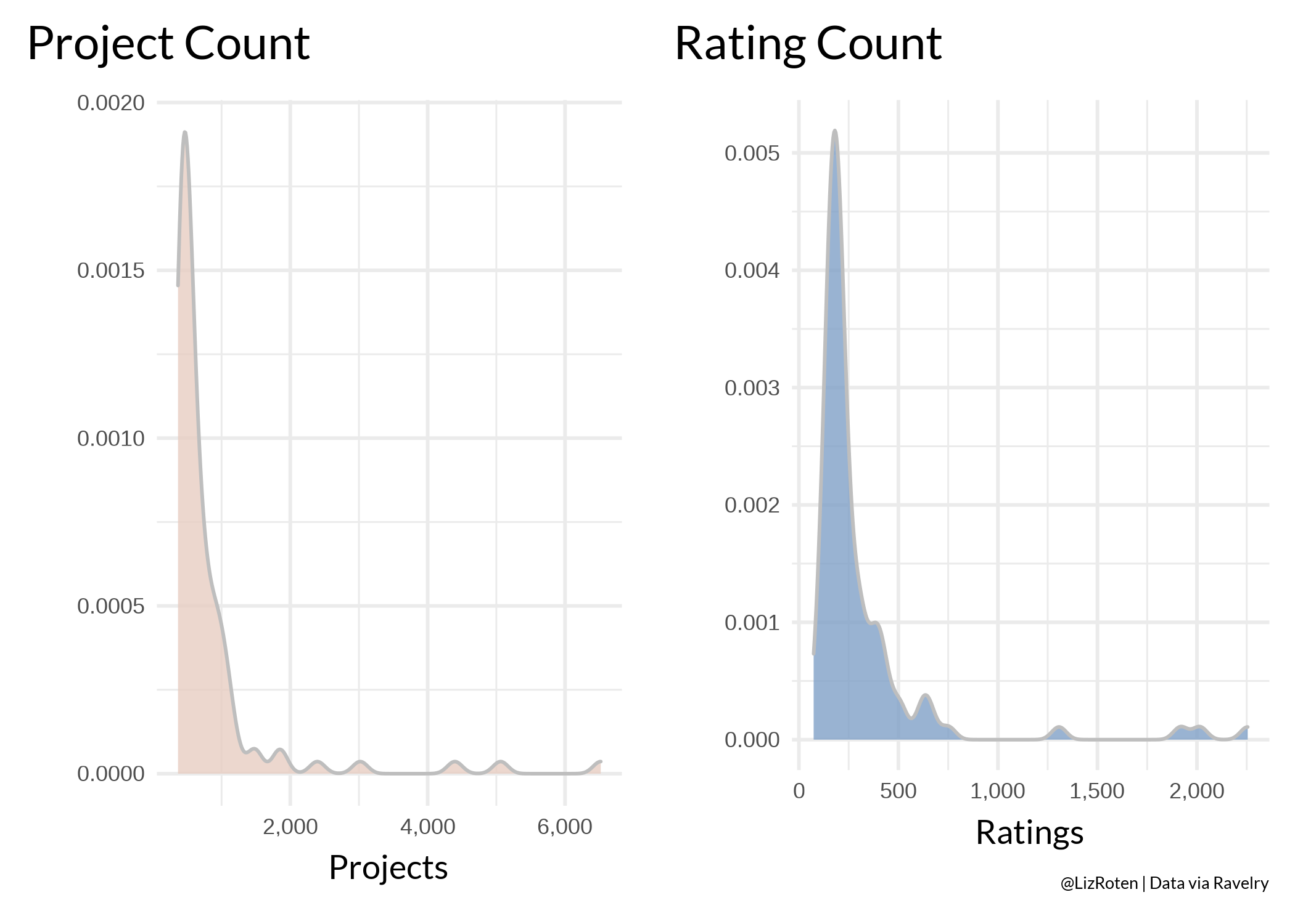
It looks like there is a big drop-off around 1,000 project and 500 ratings.
project_rating_patterns <- refined_patterns %>%
  filter(
    projects_count >= 1000,
    rating_count >= 500
  )
That filter() took us from 100 patterns to 11. Progress!
Now, lets look at the ratings and difficulty. We will also separate these out by availability.
ggplot(project_rating_patterns) +
  geom_point(
    mapping = aes(
      x = difficulty_average,
      y = rating_average,
      color = free
    ),
    size = 4
  ) +
  dutchmasters::scale_color_dutchmasters(palette = "pearl_earring") +
  labs(
    title = "Average Rating and Average Difficulty",
    x = "Average difficulty",
    y = "Average Rating",
    caption = my_caption
  ) +
  my_theme()
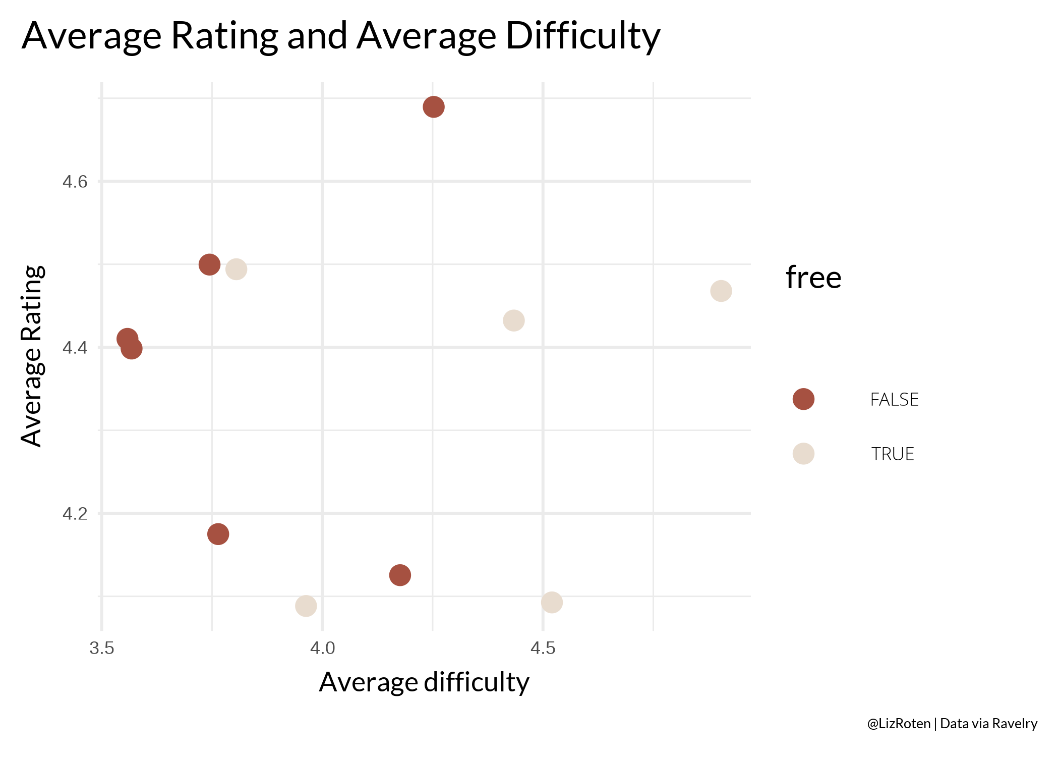
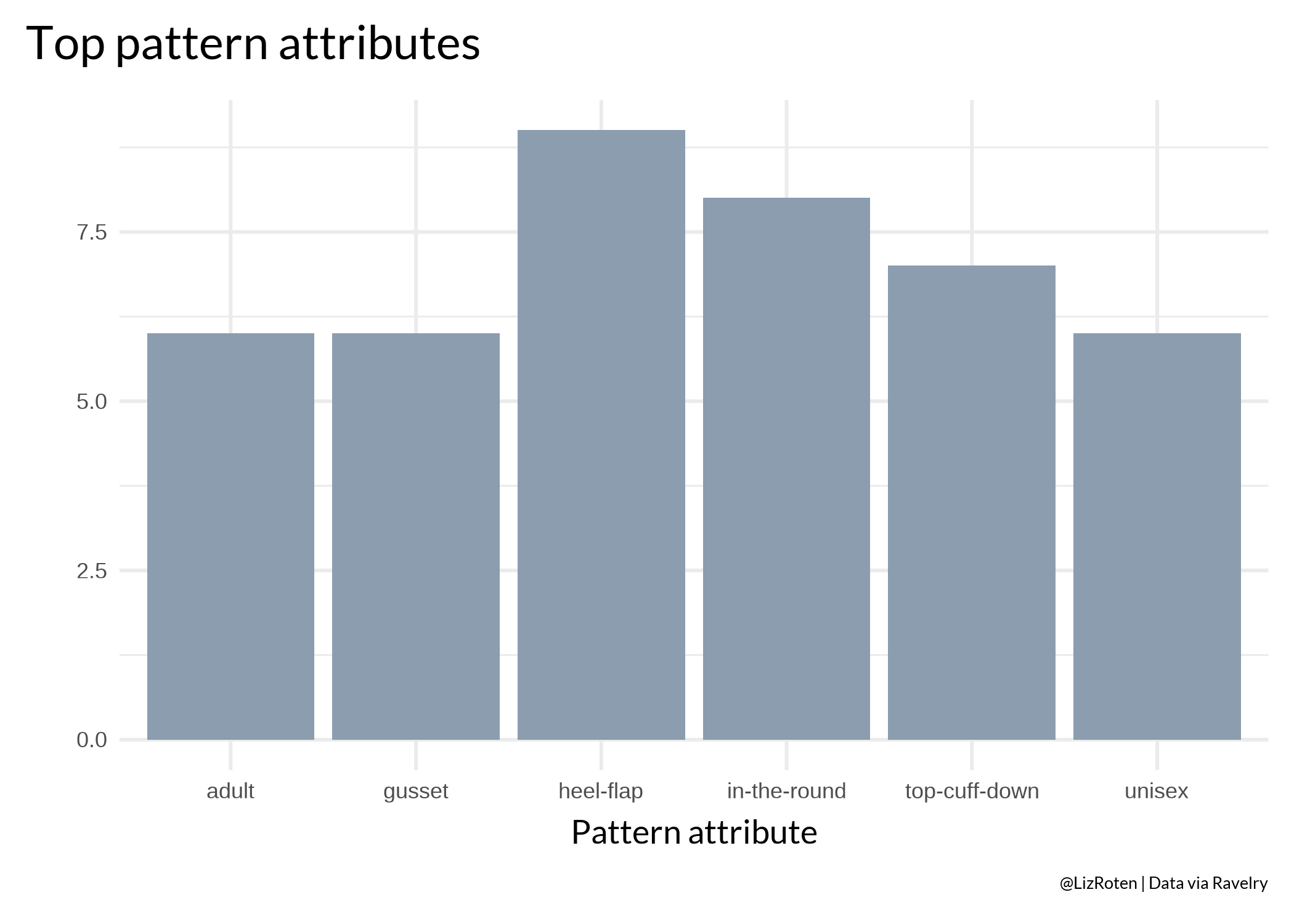
Nothing too informative here. What are the top pattern attributes?
project_rating_patterns %>%
  unnest(cols = "pattern_attributes", names_sep = "_") %>%
  count(pattern_attributes_permalink) %>%
  filter(n > 5) %>%
  arrange(desc(n)) %>%
  ggplot() +
  geom_col(aes(
    x = pattern_attributes_permalink,
    y = n
  ),
  fill = dutchmasters::dutchmasters$pearl_earring[9]
  ) +
  labs(
    title = "Top pattern attributes",
    x = "Pattern attribute",
    y = "",
    caption = my_caption

  ) +
  my_theme()
Another thing that makes patterns easy to follow is if they are downloadable (as opposed to linked to another web page). Lets filter() for that, and have a difficulty at least above 4.
filter(
  project_rating_patterns, downloadable == TRUE,
  difficulty_average >= 4
) %>%
  arrange(-rating_average)
...
#>   comments_count                created_at currency difficulty_average
#> 1              8 2010/10/25 09:23:15 -0400      USD           4.252446
#> 2             27 2007/01/12 00:51:53 -0500      USD           4.903895
#> 3            131 2010/02/11 12:07:46 -0500                    4.434030
#> 4             22 2007/09/07 11:54:33 -0400                    4.520376
#>   difficulty_count downloadable favorites_count  free gauge gauge_divisor
#> 1              511         TRUE            4027 FALSE    32             4
#> 2             2362         TRUE           11155  TRUE     8             1
...
Fetch images
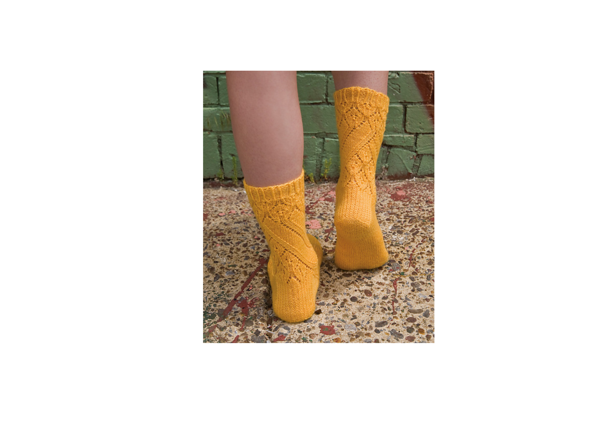
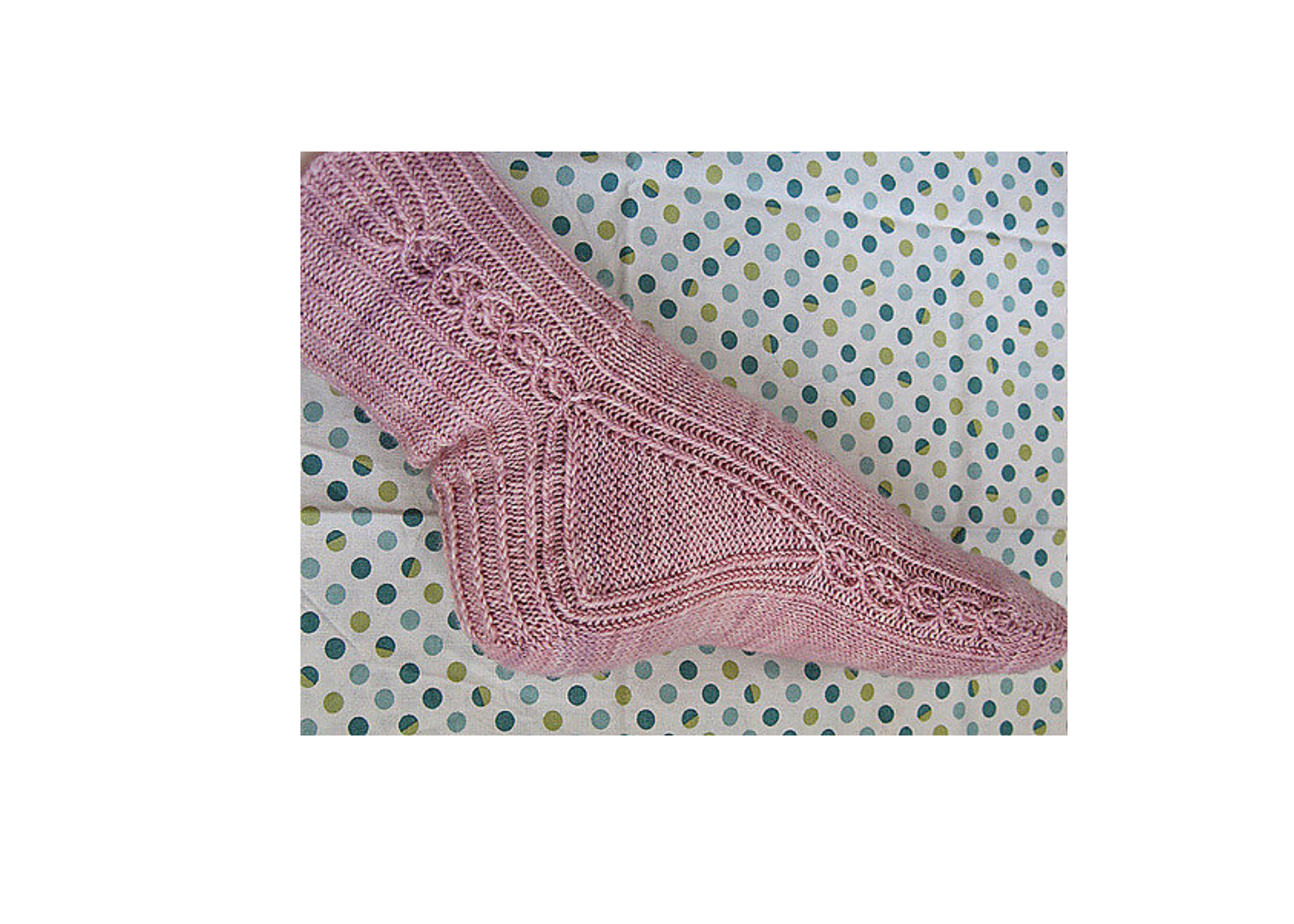
Now that we only have four left, lets fetch the images!
photo_links <- filter(
  project_rating_patterns, downloadable == TRUE,
  difficulty_average >= 4
) %>%
  unnest(cols = photos, names_sep = "_") %>%
  filter(photos_sort_order == 4) %>%
  select(id, name, photos_medium_url)
Next, we will use {imager} to fetch the data and plot it.
library(imager)
photo_links$name
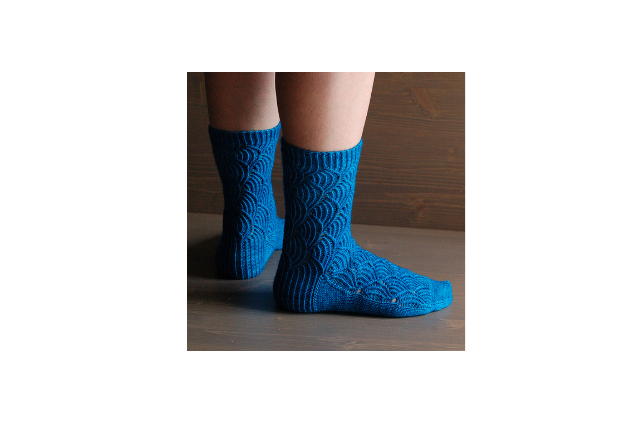
#> [1] "Pointelle"   "Firestarter" "Pomatomus"   "Skew"

map(photo_links$photos_medium_url, load.image) %>%
  map(plot, axes = FALSE)
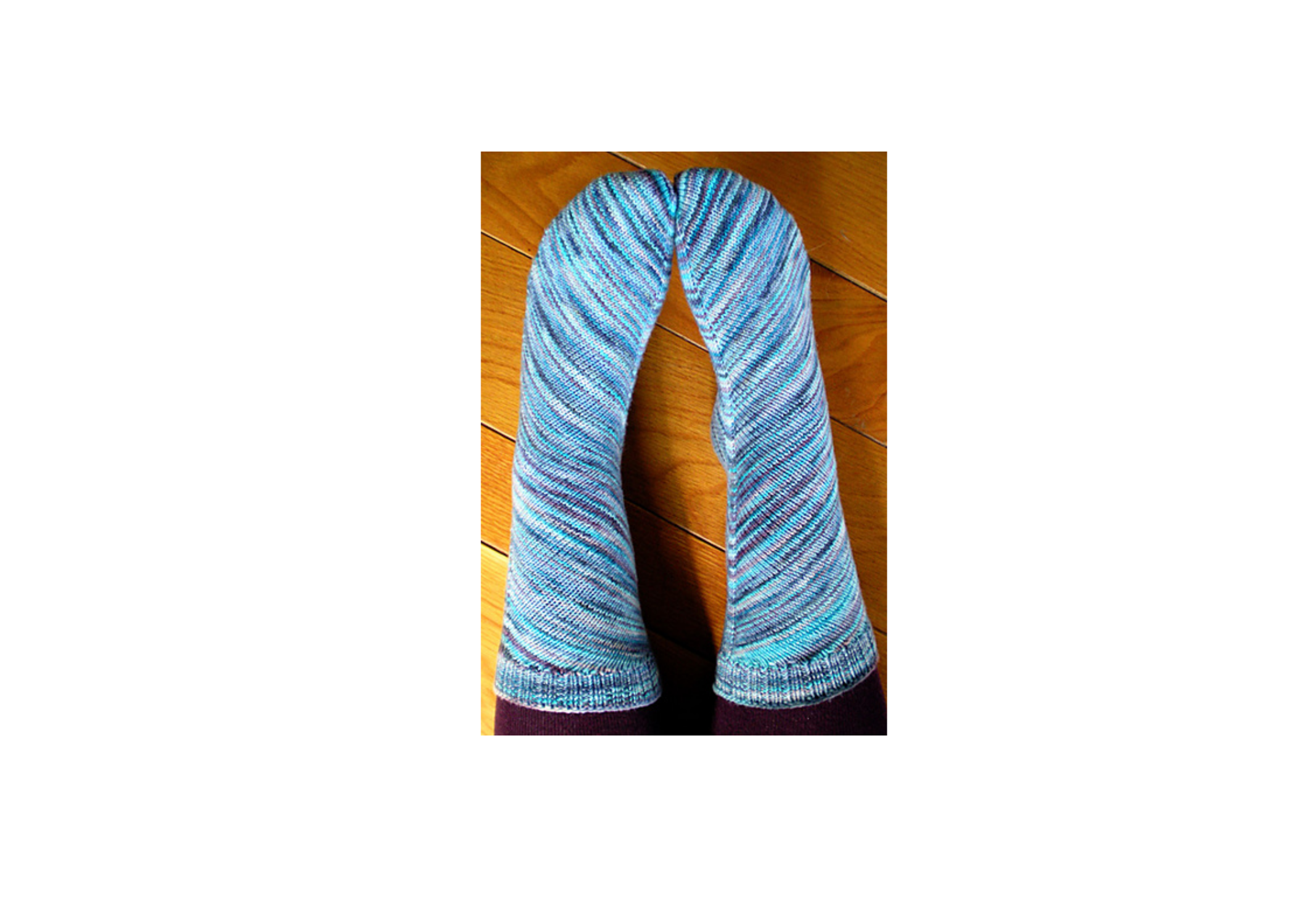
#> [[1]]
#> Image. Width: 425 pix Height: 500 pix Depth: 1 Colour channels: 3
#>
#> [[2]]
#> Image. Width: 500 pix Height: 381 pix Depth: 1 Colour channels: 3
#>
#> [[3]]
#> Image. Width: 500 pix Height: 500 pix Depth: 1 Colour channels: 3
#>
#> [[4]]
#> Image. Width: 348 pix Height: 500 pix Depth: 1 Colour channels: 3
And the winner is….
Pomatomus! I mean, look at those gorgeous waves!

I have a lovely merino/nylon blend by Sun Valley Fibers waiting for me. I hope you enjoyed this little journey!
Credits
I followed along this example by the ravelRy package author, Kaylin Pavlik. I used colors from Edwin Thoen’s R package, dutchmasters.